Landau and the dictatorship of the representation invariants
Strip away degrees of freedom, align with symmetry and achieve the dictatorship of the representation invariants.
I was attempting to recreate this paper by hand …
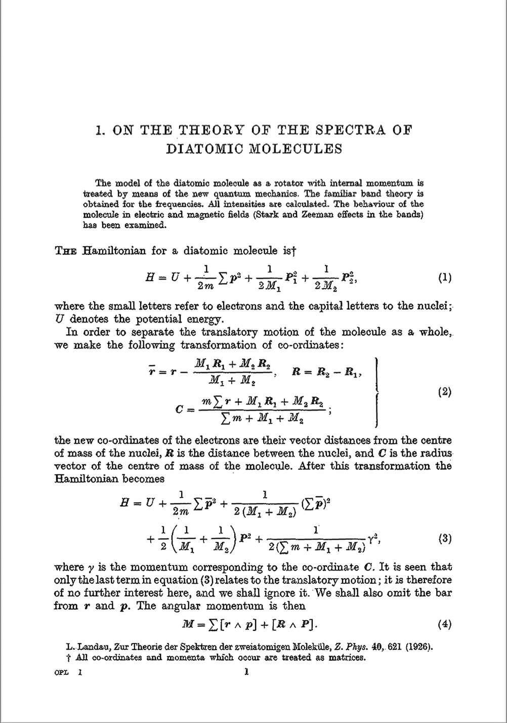 (courtesy: Collected Papers of Landau)
… and I remembered a recent article https://arxiv.org/pdf/2503.04778 on the specific method of Landau, and just was curious to test their hypothesis.
The paper “ON THE THEORY OF THE SPECTRA OF DIATOMIC MOLECULES” was written right after matrix mechanics. Spectroscopy of diatomic molecules had a well developed empirical band theory but needed a proper foundation in QM.
Step 1 - Separate the Hamiltonian in COM + relative coordinates
Letting capital letters denote the nuclei and small letters the electrons, we are given:
$$ \vec{r} = r - \frac{M_1R_1 + M_2 R_2}{M_1+M_2} \tag{1} $$ $$ R = R_2 - R_1 \tag{2} $$ $$ C = \frac{m \sum r + M_1R_1 + M_2 R_2}{ \sum m +M_1+M_2} \tag{3} $$
And instead of having $\frac{M_1R_1 + M_2 R_2}{M_1+M_2}$, let’s introduce $$ R_N = \frac{M_1R_1 + M_2 R_2}{M_1+M_2} \tag{4} $$ which is the center of mass frame of the nuclei. The expression $\vec{r} = r - R_N$ is then the electron position measured from the nuclear COM. I would prefer if he denoted it with $\vec{r}_i$ and $r_i$, indicating that we take the position of each electron and subtract the distance from the nucleus. And especially strange since we have the summation sign for the mass but not for the radius vectors.
(Just a note, in LL1 “§13 The reduced mass” you do get some basic training in two-body-problem algebra.)
To grasp equation (1) further, imagine a diatomic molecule consisisting of flourine. Each flourine atom has 9 electrons which means that $F_2$ has 18 total electrons to think about. Then the transformation $\vec{r}_i = r_i - R_N$ has to be done for every electron, i.e., we get 18 relative coordinates. What this does is to change the reference frame from the lab frame to the nuclei’s center of mass frame for every electron.
Once we get the transformed variables we want to transform the Hamiltonian. What should be our first step? Well I like to start with the momenta. Generally $\hat{p} = -i \hbar \nabla$ where $\nabla = (\frac{\partial}{\partial x}, \frac{\partial}{\partial y},\frac{\partial}{\partial z})$. So we need to express $\nabla_{R_1}$, $\nabla_{R_2}$ and $\nabla_{r}$ in $C, R$ and $\vec{r_i}$.
We start by rewriting $R_1$ and $R_2$ in terms of the new variables. For $R_1$ we plug $R_2 = R+R_1$ into eq. 4:
$$ R_N = \frac{ M_1R_1 + M_2(R+R_1)}{+M_1+M_2} = \frac{R_1(M_1+M_2)+M_2R}{M_1+M_2} $$
$$ = R_1 + \frac{M_2}{M_1+M_2}R \leftrightarrow R_1 = R_N - \frac{M_2}{M_1+M_2}R $$
Similarly for $R_2$ we do the same procedure but with $R_1 = R_2-R$ into eq. 4 $$ R_N = \frac{ M_1(R_2-R) + M_2 R_2}{+M_1+M_2} = \frac{R_2(M_1+M_2)-M_1R}{M_1+M_2} $$
$$ = R_2 - \frac{M_1}{M_1+M_2}R \leftrightarrow R_2 = R_N + \frac{M_1}{M_1+M_2}R $$
And for the electron lab frame vector we have $r = \vec{r} + R_N$ from eq. (1), and rewriting this in terms of $C$:
$$ r = \vec{r} + C - \frac{m}{\sum m + M_1 + M_2} \sum \vec{r} $$
$$ R_1 = C - \frac{m \sum \vec{r}}{\sum m+ M_1+M_2} - \frac{M_2}{M_1+M_2}R $$
$$ R_2 = C - \frac{m \sum \vec{r}}{\sum m+ M_1+M_2} + \frac{M_1}{M_1+M_2}R $$
Now we want to derive the expressions for $\nabla_{R_1}$, $\nabla_{R_2}$ and $\nabla_{r}$. Recall that the multivariable chain rule for a function $f(x(q))$: $\frac{\partial f}{\partial q_i} = \sum_j \frac{\partial x_j}{\partial q_i} \frac{\partial f}{\partial x_j}$. Set $\alpha := \frac{m}{\sum m + M_1 + M_2}$.
Computing $\nabla_{r}$: $$ \nabla_r = \frac{\partial \vec{r}}{\partial r} \nabla_{\vec{r}} + \frac{\partial R}{\partial r} \nabla_{R} + \frac{\partial C}{\partial r} \nabla_{C} $$ $$ = \nabla_{\vec{r}} + \alpha \nabla_{C} $$
Computing $\nabla_{R_1}$: $$ \nabla_{R_1} = \frac{\partial C}{\partial R_1} \nabla_{C} + \frac{\partial \vec{r}}{\partial R_1} \nabla_{\vec{r}} + \frac{\partial R}{\partial R_1} \nabla_{R} $$ $$ = \frac{M_1}{\sum m + M_1 + M_2} \nabla_C - \sum \frac{M_1}{M_1+M_2}\nabla_{\vec{r}} + (-1) \nabla_{R} $$ Computing $\nabla_{R_2}$: $$ \nabla_{R_2} = \frac{\partial C}{\partial R_2} \nabla_{C} + \frac{\partial \vec{r}}{\partial R_2} \nabla_{\vec{r}} + \frac{\partial R}{\partial R_2} \nabla_{R} $$ $$ = \frac{M_2}{\sum m + M_1 + M_2} \nabla_C - \sum \frac{M_2}{M_1+M_2}\nabla_{\vec{r}} + \nabla_{R} $$
(Note to self: when $\nabla_{\vec{r}}$ appears in $\nabla_{R_{1,2}}$)
Computing the momenta
From the text we can deduce $P_1 = -i \hbar \nabla_{R_1}, P_2 = -i \hbar \nabla_{R_2},$ and $p_r = -i \hbar \nabla_r$. Properly expressed in new variables:
$$ p_i = -i\hbar (\nabla_{\vec{r}} + \alpha \nabla_C) $$ $$ P_1 = -i\hbar (\frac{M_1}{\sum m + M_1 + M_2} \nabla_C - \sum \frac{M_1}{M_1+M_2}\nabla_{\vec{r}} - \nabla_{R}) $$ $$ P_1 = -i\hbar (\frac{M_2}{\sum m + M_1 + M_2} \nabla_C - \sum \frac{M_2}{M_1+M_2}\nabla_{\vec{r}} + \nabla_{R}) $$
Set $\gamma = -i \hbar \nabla_C$, $p_{\vec{r}} = -i \hbar \nabla_{\vec{r}}$ and $P_{R} = -i \hbar \nabla_{R}$
Now we want to compute each term in the kinetic energy given in the first equation.
$$ p^2_i = p^2_{\vec{r}} + 2 \alpha p_{\vec{r}} \gamma + \alpha^2 \gamma^2 $$
$$ \implies \frac{1}{2m} \sum p^2_i = \frac{1}{2m}(\sum p^2_{\vec{r}}) + 2 \alpha \gamma \sum p_{\vec{r}} + \alpha^2 \gamma^2 \sum_i * 1) $$
For the $P_1$ term
$$ P_1 = \frac{M_1}{\sum m + M_1 + M_2 }\gamma - \frac{M_1}{M_1+M_2} \sum p_{\vec{r}} - P_R $$
$$ \implies P^2_1 = (\frac{M_1}{\sum m + M_1 + M_2 }\gamma)^2 + (- \frac{M_1}{M_1+M_2} \sum p_{\vec{r}})^2 + (-P_R)^2 + … $$
$$ … + 2(\frac{M_1}{\sum m + M_1 + M_2 }\gamma)(- \frac{M_1}{M_1+M_2} \sum p_{\vec{r}}) + 2(\frac{M_1}{\sum m + M_1 + M_2 }\gamma)(-P_R) + … $$
$$ … + 2(- \frac{M_1}{M_1+M_2} \sum p_{\vec{r}})(-P_R) $$
And therefore
$$ \frac{P_1^2}{2M_1} = \frac{M_1}{2(\sum m + M_1 + M_2)^2}\gamma^2+\frac{M_1}{2(M_1+M_2)^2}(\sum p_{\vec{r}})^2 + \frac{1}{2M_1}P_R^2 + … $$
$$ … -\frac{M_1}{(M_1+M_2)(\sum m + M_1 + M_2)}(\sum p_{\vec{r}})\gamma - \frac{1}{\sum m + M_1 + M_2}\gamma P_R + … $$ $$ … + \frac{1}{M_1+M_2}(\sum p_{\vec{r}})P_R $$
For the $P_2$ term:
$$ P_2 = \frac{M_2}{\sum m + M_1 + M_2 }\gamma - \frac{M_2}{M_1+M_2} \sum p_{\vec{r}} + P_R $$
$$ \implies P^2_2 = (\frac{M_2}{\sum m + M_1 + M_2 }\gamma)^2 + (- \frac{M_2}{M_1+M_2} \sum p_{\vec{r}})^2 + P_R^2 + … $$
$$ … + 2(\frac{M_2}{\sum m + M_1 + M_2 }\gamma)(- \frac{M_2}{M_1+M_2} \sum p_{\vec{r}}) + 2(\frac{M_2}{\sum m + M_1 + M_2 }\gamma)(P_R) + … $$ $$ … + 2(- \frac{M_2}{M_1+M_2} \sum p_{\vec{r}})(P_R) $$
And therefore
$$ \frac{P_2^2}{2M_2} = \frac{M_2}{2(\sum m + M_1 + M_2)^2}\gamma^2+\frac{M_2}{2(M_1+M_2)^2}(\sum p_{\vec{r}})^2 + \frac{1}{2M_2}P_R^2 + … $$
$$ … -\frac{M_2}{(M_1+M_2)(\sum m + M_1 + M_2)}(\sum p_{\vec{r}})\gamma + \frac{1}{\sum m + M_1 + M_2}\gamma P_R + … $$ $$ … - \frac{1}{M_1+M_2}(\sum p_{\vec{r}})P_R $$
Finally we can start comparing terms now, for the $\sum p_{\vec{r}} \cdot P_R$: $$ \frac{1}{M_1+M_2} - \frac{1}{M_1+M_2} = 0 $$
and for $\gamma \cdot P_R$: $$ -\frac{1}{\sum m + M_1 + M_2} + \frac{1}{\sum m + M_1 + M_2} = 0 $$
and for $\sum p_{\vec{r}} \cdot \gamma$:
$$ -\frac{M_1}{(M_1+M_2)(\sum m + M_1 + M_2)} - \frac{M_2}{(M_1+M_2)(\sum m + M_1 + M_2)} = $$
$$ = -\frac{1}{\sum m + M_1 + M_2} $$ (which will cancel with the electron part)
for $\sum p_{\vec{r}}^2$: $$ \frac{M_1}{2(M_1+M_2)^2} + \frac{M_2}{2(M_1+M_2)^2} = \frac{1}{2(M_1+M_2)} $$ and for $P^2$: $$ \frac{1}{2M_1} + \frac{1}{2M_2} $$
and for $\gamma^2$: $$ \frac{M_1+M_2}{2(\sum m + M_1 + M_2)^2} $$
Alas the kinetic energy becomes:
$$ \frac{1}{2m}(\sum p^2_{\vec{r}} + 2 \alpha \gamma \sum p_{\vec{r}} + \alpha^2 \gamma^2 \sum_i) - \frac{1}{\sum m + M_1 + M_2} (\sum p_{\vec{r}})\gamma + … $$
$$ … + \frac{1}{2(M_1+M_2)}(\sum p^2_{\vec{r}}) + (\frac{1}{2M_1}+ \frac{1}{2M_2})P^2_R + \frac{M_1+M_2}{2(\sum m + M_1+M_2)^2}\gamma^2 $$
To simplify this we notice that the electron cross term $\frac{1}{2m} 2\alpha \gamma \sum p_{\vec{r}} = \frac{1}{\sum m + M_1 + M_2} \gamma \sum p_{\vec{r}}$ cancels exactly with the nuclear cross term: $- \frac{1}{\sum m + M_1 + M_2} (\sum p_{\vec{r}})\gamma$. And lastly, since $\sum_i = \frac{\sum m}{m}$, then from the electron part: $\frac{1}{2m} \alpha^2 \gamma^2 \frac{\sum m}{m} = \frac{1}{2m} (\frac{m}{\sum m + M_1 + M_2})^2 \gamma^2 \frac{\sum m}{m} = \frac{\gamma^2}{(\sum m + M_1 + M_2)^2} \sum m$. Adding the $\gamma^2$ from the nuclear part:
$$ (\frac{\sum m}{(\sum m + M_1 + M_2)^2} + \frac{M_1+M_2}{2(\sum m + M_1+M_2)^2})\gamma^2 = $$ $$ = \frac{2\sum m + M_1+M_2}{2(\sum m + M_1+M_2)^2}\gamma^2 = \frac{1}{(\sum m + M_1+M_2)^2}\gamma^2 $$
Super! The finalized result for the kinetic energy is then:
$$ \frac{1}{2m} \sum p^2_{\vec{r}} + \frac{1}{2(M_1+M_2)}(\sum p_{\vec{r}})^2 + \frac{1}{2}(\frac{1}{M_1}+ \frac{1}{M_2})P^2_R + \frac{1}{(\sum m + M_1+M_2)^2}\gamma^2 $$
Which is the exact result presented in equation (3) in the paper.
The $\gamma$ term is corresponding to the motion of the molecule’s COM. However, the spectra does not depend on how the molecule is moving through space, and the motion is separable from internal motion, i.e., $\Psi = \Psi(r,R) \cdot \Psi_{CM}(C)$ and this is why Landau says that “of no further interest here, we ignore it.” Nothing would change if we kept the term around for the next step, but recognizing this allows us to not carry around unnecessary baggage.
Step 2 - Describe the molecule’s rotation
The first question to ask now is why is Landau introducing angular momentum?
I think the answer is the following: For a system in an external field we cannot claim that the angular momentum is conserved. But if there is a symmetry, e.g., centrally symmetric field or as in this problem an “axially” symmetric field (later explain what that means) then the component of angular momentum along the axis of symmetry is conserved. But how do we even show that the corresponding conserved quantity is precisely this?
Think about the Hamiltonian of a closed system. By closed system we mean “a system of particles which interact with one another but with no other bodies.” (See the definition in LL1 “§5. Lagrangian for a system of particles.”) You might object, “well, isn’t the diatomic molecule a closed system? And if that is the case then why are we bothering with axial symmetry?” Yes, the diatomic molecule is a closed system. But we switched to relative coordinates and in this case only the projection along the axis of the molecule is constant. Remember, Landau teaches us that the angular momentum of a system depends on the point with respect to which it is defined. Why? Because angular momentum involves the radius vector. And for a rigid body, the most fitting point is the COM of the body.
The reason why we understand that it has to be angular momentum that becomes conserved instead of any other quantity is the following: Due to the isotropy of space we have a condition for an infinitely small rotation that eventually becomes:
$$ (\sum_a r_a \times \nabla_a )\hat{H} - \hat{H}(\sum_a r_a \times \nabla_a) = 0 \tag{§26 QM} $$
(Might be relevant here to learn how to do this small rotation reasoning leading to this condition, e.g., check LL1 “§9” for steps. Also, I believe this is a problem in Kotkin & Serbo Collection of Problems in Classical Mechanics in the ch. on angular momentum. This is important to know if you want to pass the modern Landau exam in CM.)
And this quantity we call the angular momentum. Now that we have some slight understanding to why AM shows up, let’s proceed more concretely.
In the second (revised) edition 1965 of Vol. 3 in A course in theoretical physics, §82 part of the ch. The Diatomic molecule, there is an eerily similar problem to what Landau actually does in this paper. The problem is stated as follows:
“Determine the angular part of the wave function for a diatomic molecule with zero spin (F. Reiche 1926)”
But this is solved in a completely different way than what he did in this paper. So at this junction, we have the possibility to treat the problem in two different ways! And even more strangely, in the physical copy of Vol. 3 (3rd edition) that I have, the first problem for §82 is not the above but something completely different, it is about determining the accuracy of the approximation which gives the separation of the electrons and nuclear motions in the diatomic molecule. I have no idea why they changed this.
Moving to the 2nd page of the paper, Landau starts out by switching to spherical coordinates, by denoting $\vec{R} = (R, \theta, \phi)$ we now need to express the operators of angular momentum of this form.
Generally we know: $$ \hat{l}_z = -i \frac{\partial}{\partial \phi} $$
$$ \hat{l}_{\pm} = e^{\pm i \phi}(\pm \frac{\partial}{\partial \theta}+ i \cot \theta \frac{\partial}{\partial \phi}) $$
How do we arrive at these results? He calls it a “simple calculation” and omits the details, but … here’s the solution for $\hat{l}_z$: Given $r = (x,y,z)$ and $p = (p_x, p_y, p_z)$ we get $\hat{l} = \hat{x}(yp_z-zp_y) -\hat{y}(xp_z-zp_x) + \hat{z}(xp_y-yp_x)$. And now we need to express each $\nabla_x, \nabla_y$ and $\nabla_z$ in spherical coordinates. Keep in mind that $r = \sqrt{x^2+y^2+z^2}$, $\theta = \arccos{\frac{z}{r}}$ and $\phi = \arctan{\frac{y}{x}}$. To find $\hat{l}_z$ we need to compute $\nabla_y$ and $\nabla_x$ :
$$ \nabla_y = \frac{1}{\partial r} \frac{\partial r}{\partial y} + \frac{1}{\partial \theta} \frac{\partial \theta}{\partial y} + \frac{1}{\partial \phi} \frac{\partial \phi}{\partial y} $$
Clearly $\frac{\partial r}{\partial y} = \frac{y}{\sqrt{x^2+y^2+z^2}}$, $\frac{\partial \theta}{\partial y} = -\frac{1}{\sqrt{1-u^2}} \frac{\partial u(y)}{\partial y} = -\frac{1}{\sqrt{1-u^2}} (-1)\frac{zy}{(x^2+y^2+z^2)^{3/2}} = \frac{1}{\sqrt{1-\frac{z^2}{r^2}}}\frac{zy}{r^3}$ and $\frac{\partial \phi}{\partial y} =\frac{1}{1+(\frac{y}{x})^2} \frac{1}{x} = \frac{x}{x^2+y^2}$
For $$ \nabla_x = \frac{1}{\partial r} \frac{\partial r}{\partial x} + \frac{1}{\partial \theta} \frac{\partial \theta}{\partial x} + \frac{1}{\partial \phi} \frac{\partial \phi}{\partial x} $$
$\frac{\partial r}{\partial x} = \frac{x}{\sqrt{x^2+y^2+z^2}}$, $\frac{\partial \theta}{\partial x} = -\frac{1}{\sqrt{1-u^2}} \frac{\partial u(x)}{\partial x} = \frac{1}{\sqrt{1-\frac{z^2}{r^2}}} \frac{xz}{r^3} $ and $\frac{\partial \phi}{\partial x} =\frac{1}{1+(\frac{y}{x})^2}(-1) \frac{y}{x^2} = -\frac{y}{x^2+y^2}$
$$ \hat{l}_z = xp_y-yp_x = x(\frac{y}{r}\nabla_r+\frac{1}{\sqrt{1-\frac{z^2}{r^2}}}\frac{zy}{r^3}\nabla + \frac{x}{x^2+y^2}\nabla) - y(\frac{x}{r}\nabla + \frac{1}{\sqrt{1-\frac{z^2}{r^2}}} \frac{xz}{r^3}\nabla-\frac{y}{x^2+y^2}\nabla) $$
$$ = \frac{x^2+y^2}{x^2+y^2}\nabla_{\phi} = \nabla_{\phi} \implies \hat{l}_z = -i \frac{\partial}{\partial \phi} $$ (with $\hbar = 1$.)
Anyway, moving on, we need to express $\vec{R}$ in $R, \theta$ and $\phi$. The square of the angular momentum operator $L$ is
$$ \hat{L}^2 = L_-L_+ + L^2_z + L_z $$
Subbing the expressions for $l_{\pm}$ and $l_z$ into the above yields:
$$ \hat{l}^2 = -\hbar^2[\frac{1}{\sin^2 \theta} \frac{\partial^2}{\partial \phi^2}+\frac{1}{\sin \theta} \frac{\partial}{\partial \theta}(\sin \theta \frac{\partial}{\partial \theta})] $$
s.t., $P^2_R = -\hbar^2 \nabla^2_R = p^2_R + \frac{1}{R^2} \hat{l}^2$. Let’s see if we can identify the $p_\theta$ and $p_\phi$ from this expression. First thing to keep firm in your mind is that operators corresponding to physical quantities need to be Hermitian.
Hermiticity condition for an operator $\hat{A}$ is
$$ \int (\hat{A} \Psi^{+})\Psi dq = \int \Psi^{+} \hat{A} \Psi dq $$
for $p_R = -i\hbar \frac{\partial}{\partial R}$:
$$ \int_0^∞ f* p_R* gR^2dR = \int_0^∞ f -i\hbar \frac{\partial}{\partial R}gR^2dR $$